Every BLDC motor behind a geared robot joint carries one number that quietly shapes everything else on the page: the reduction ratio. The ratio multiplies torque, divides speed, and — through a square law that most datasheets never spell out — scales the reflected inertia on both sides of the gear mesh. This guide works through the arithmetic with published figures from real actuator pages, then turns it into a sizing sequence for a robot joint.
What a Reduction Ratio Does to Torque and Speed
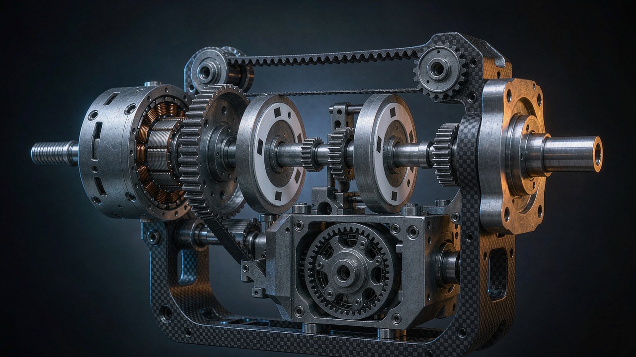
A planetary gearbox sits between the rotor and the joint, and the reduction ratio describes how many times the rotor turns for one turn of the output. A 10:1 reduction ratio means ten rotor revolutions per output revolution. In the ideal, lossless picture the exchange is exact: torque at the output is motor torque multiplied by the ratio, and speed at the output is motor speed divided by it. Multiply torque by ten, divide speed by ten, and the mechanical power flowing through the joint stays where the electrical side put it.
Real gears are not lossless. Each planetary stage carries mesh losses, bearing drag and churning losses, so the torque arriving at the output falls short of what the reduction ratio promises on paper. Datasheets absorb those losses into the rated and peak torque rows, which is why the published figures are already output-side numbers: the CubeMars AK80-64 publishes 48 Nm of rated torque and 120 Nm of peak torque at the output flange, behind its 64:1 stage, not at the rotor. The honest way to read a geared actuator page is therefore to treat every torque and speed row as post-gearbox, and to treat the electrical rows — current, voltage, the torque constant — as pre-gearbox.
The reduction ratio also hides in plain sight in the model names on the CubeMars AK and AKH lines: an AK45-10 carries a 10:1 stage, an AK45-36 a 36:1 stage, an AKH70-48 a 48:1 stage. Reading the number out of the name before opening the page is a habit worth forming, because the reduction ratio is the one specification that every other output-side row inherits.
The output side of the gearbox
That split matters because two pages that look identical describe different machines once the reduction ratio enters. The rotor inside the AK80-64 turns at up to 4800 rpm to deliver the 75 rpm published at the output; the encoder on the motor shaft counts 64 rotor turns per output turn. When a selection guide compares a direct drive frameless kit against an integrated geared module, the comparison only lands if both sides are stated at the same shaft. The torque-speed curve article on this site covers how the electrical limit shapes the raw motor curve; the present piece stays on the far side of the gear mesh, where the joint actually lives and where reflected inertia is felt.
The low-ratio end of the trade has its own economics. A quasi direct drive module keeps the reduction ratio near single digits — the CubeMars AKE series sits at 6:1 and 8:1 — and pays for that with lower output torque but a lighter, more transparent drivetrain. What an 8:1 stage buys in backdrivability and force transparency, and what it costs in torque, is worked through in Quasi Direct Drive Actuators: What an 8:1 Ratio Buys You; the present guide covers the general rule that the QDD philosophy pushes against.
Where the multiplication stops being free
Torque multiplication also shifts where the operating point sits on the motor curve. A joint that needs 24 Nm of continuous torque does not need a motor that makes 24 Nm — it needs a motor whose continuous torque, times the ratio, times the stage efficiency, clears 24 Nm while its current draw stays inside the thermal budget. The thermal side of that budget, and how a torque-speed curve separates continuous from peak operation, is covered in Continuous Torque vs Peak Torque: Duty Cycle, Thermal Limit, Torque-Speed Curve. The gearbox cannot multiply what the winding cannot sustain, and the reflected inertia it adds is the second half of the same bill.
Reflected Inertia: The Square Law at the Gearbox
The reduction ratio trades speed for torque at a linear exchange rate. Inertia does not play by that rule. Any inertia on one side of a gearbox appears on the other side multiplied or divided by the square of the ratio, and that single fact organizes the whole sizing problem. Engineers call the transformed value the reflected inertia: the inertia a component would need to have, sitting directly on the shaft being analyzed, to produce the same dynamic behavior. This relation is the kinematic one for an ideal rigid transmission — mesh compliance, elasticity and losses inside the stages shift it in detail, and the places where those second-order effects matter are flagged along the way. Both transformations run through the reduction ratio, which is why ratio selection is an inertia decision as much as a torque decision.
Why the rotor grows by the square
Start at the output and look back at the motor. The reflected inertia of the rotor, seen at the output shaft, is the rotor inertia multiplied by the square of the reduction ratio. The arithmetic is unforgiving: square a small ratio and almost nothing happens; square a large one and the numbers explode. A 6:1 stage multiplies rotor inertia by 36. A 64:1 stage multiplies it by 4096. Reflected inertia is therefore not a refinement that only analysts care about — between a 6:1 and a 64:1 module it is a factor of more than one hundred on the same physical rotor.
The published CubeMars AKH70 pair makes the square law measurable through a same-rotor comparison — not a strict single-variable test, since the stage count and the transmission efficiency change along with the ratio, but the closest thing a datasheet offers. The AKH70-16 and the AKH70-48 share one rotor: both pages publish the same rotor inertia of 1170 g·cm², the same KV41 winding, the same 90 mm housing. The only meaningful difference is the gearbox — a two-stage 16:1 unit on one, a three-stage 48:1 unit on the other. Reflect each rotor to its own output and the shared part becomes two different machines: 16 squared is 256, and 256 × 1170 g·cm² is 299520 g·cm² of reflected inertia at the output of the AKH70-16; 48 squared is 2304, and 2304 × 1170 g·cm² is 2695680 g·cm² at the output of the AKH70-48. Tripling the ratio multiplied the reflected inertia by nine.
That is the real price list for high ratios. The AKH70-48 delivers 74 Nm of rated torque against 26 Nm for the AKH70-16 — a factor of 2.85 — while the reflected inertia of that same rotor, seen at the output shaft, grew by a factor of nine. Peak torque tells the same story: 222 Nm against 78 Nm. When a joint designer reads a high-ratio module as a small motor with a magic multiplier, the square law on reflected inertia is the correction.
Why the load shrinks by the square
The same law runs in reverse, and this direction is the useful one. A load inertia on the output shaft, seen from the motor shaft, is divided by the square of the reduction ratio. A heavy robot leg that presents 0.005 kg·m² at the hip looks like a tenth of that to the rotor behind a 10:1 stage, because the rotor only has to accelerate its share of the motion — one ratio-squared slice of it. The reflected inertia of the load is a much smaller number than the load sitting still at the joint.
This is why geared joints drive arms and legs that a bare motor could not move dynamically. The gearbox does not just make torque affordable; it shrinks the reflected inertia of the load until the rotor can dominate the acceleration budget. And the two square-law effects meet in the middle: rotor inertia grows toward the output, load inertia shrinks toward the motor, and the reduction ratio that balances the two is the subject of the next section.
The AK45 pair as a second data point
The AKH70 pair is the cleanest comparison because the rotor is shared. The AK45 family repeats the pattern at a smaller frame with two different rotors. The AK45-10 publishes a rotor inertia of 157.33 g·cm² behind a 10:1 stage, which reflects to 15733 g·cm² at the output; the AK45-36 publishes 181.9 g·cm² behind 36:1, which reflects to 235742.4 g·cm². Moving from 10:1 to 36:1 inside the same family multiplied the reflected inertia by roughly fifteen, while rated torque moved from 2.5 Nm to 8 Nm and no-load speed fell from 180 rpm to 52 rpm. The 36:1 module delivers a little more than three times the rated torque, at roughly fifteen times the output-side reflected inertia and 87 g of additional mass.
Inertia Matching: The Load-to-Rotor Inertia Ratio
Put the two square-law effects side by side and a single dimensionless number falls out: the load-to-rotor inertia ratio, computed at one shaft. Divide the reflected load inertia by the rotor inertia plus the gearbox inertia, all referenced to the same side, and the inertia ratio says how much of the motor torque is spent accelerating the load versus accelerating its own rotating parts. Inertia matching is the practice of keeping that ratio inside a band the control loop can live with. Reflected inertia is the currency both sides are counted in.
Reading the inertia ratio on a datasheet
On an integrated actuator page the computation is short because the manufacturer publishes the rotor inertia. Take the AKH70-16 driving a hip load: the load inertia reflected to the motor shaft is the joint inertia divided by 256, and the rotor contributes 1170 g·cm² directly. The inertia ratio is the first divided by the second. CubeMars prints rotor inertia for the AK, AKH and AKE lines, so a buyer can run this check from the published pages alone — no teardown, no guesswork. That published row is the single most under-used number on an actuator datasheet, and it is the only input the inertia ratio needs that a torque table does not already provide. A check built on it is a first-pass estimate: a complete model would add the gearbox inertia reflected to the same shaft, together with any transmission compliance the application is sensitive to.
One convention decision makes the arithmetic shorter: pick a shaft and stay on it. Computing at the motor shaft keeps the rotor inertia as printed and divides the load by the square of the stage; computing at the joint shaft keeps the load as measured and multiplies the rotor by the same square. The reflected inertia differs by that factor between the two shafts, but the inertia ratio comes out identical either way — mixing reference points mid-calculation is the most common slip in a first sizing pass.
What a mismatched joint feels like
When the inertia ratio runs high — a heavy load behind a comparatively light rotor — the joint becomes a tuning problem before it becomes a strength problem. The load dominates the frequency response, and combined with gearbox compliance and limited damping it can pull mechanical resonances toward the control bandwidth and stretch settling time. Gains have to drop, and the joint feels sluggish in exactly the way the torque numbers said it would not.
When the inertia ratio runs very low, the opposite waste appears: the joint spends its current accelerating its own rotor and gears, and torque capability at the joint goes unused — the design may carry more motor than the motion needs, though some applications deliberately favor a larger rotor inertia for dynamic or control reasons. The mass budget pays for a rotor big enough to dwarf the load — sometimes the right call, as the next subsection shows, but never a free one.
The inertia ratio therefore works as a sanity band rather than a target digit. Selection practice across servo literature keeps the reflected load within a modest multiple of the rotor inertia, and the exact ceiling depends on the control loop, the stiffness of the mounting and how much settling time the application tolerates. A collaborative arm settling to a stable position cares differently from a leg joint absorbing impacts at footfall. What the datasheet gives is the inputs; where the band sits is an application decision. Inertia matching, not the inertia ratio itself, is the discipline — the number is simply where the discipline is measured.
When to relax the target
Two situations justify stepping outside a comfortable inertia ratio. The first is impact: a legged robot joint that takes ground strikes through its output responds differently when the rotor is large relative to the load, because the reflected rotor inertia at the output reshapes how the drivetrain reacts to the strike. Impacts still call for a separate dynamic assessment — contact stiffness, gearbox stiffness and damping, joint compliance and the controller all shape how impact energy travels through the gear train — so a large reflected rotor inertia is not by itself protection for the gear teeth. The second is force transparency: an exoskeleton joint that the operator must backdrive by hand wants the smallest possible ratio and the lightest possible rotor, which is exactly the quasi direct drive argument. Both are covered from the application side in BLDC Motors for Humanoid Robot: How to Match Torque, Speed and Size.
What a High Reduction Ratio Costs: Speed Ceiling, Backlash and Mass
A high reduction ratio is bought, not given. Three costs appear on the datasheet itself — a speed ceiling, backlash, and mass — and a fourth, the square-law reflected inertia from the previous section, only appears once the arithmetic is done. The inertia ratio a joint ends up with is set by the same dial, because the ratio that grows the reflected inertia of the rotor is the one that shrinks the reflected load.
The speed ceiling
The reduction ratio divides rotor speed by the same factor it multiplies torque, so a high ratio caps joint velocity at the output. The AK45-36 publishes 52 rpm of no-load speed against 180 rpm for the AK45-10; the AKH70-48 publishes 35 rpm against 105 rpm for the AKH70-16. A wrist joint that must spin several turns per second cannot use the ratio that its torque demand suggests, and the constraint binds before the torque margin does. Voltage moves the ceiling somewhat — the AK80-64 publishes 23 rpm of rated speed on a 24 V bus and 48 rpm on 48 V, from the same 64:1 stage — and the system-level consequences of running the higher bus are covered in 48 V Robotic Actuators: Models, Performance Benefits, and System Constraints. A gear ratio is a commitment to a ceiling; choosing the reduction ratio is choosing the ceiling.
Backlash and the accuracy budget
Every gear mesh carries a small amount of free play, published as backlash. The figures are small and unit-sensitive: the AK45-10 page prints 18 arcmin, the AK45-36 and both AKH70 modules print 12 arcmin, and the AK80-64 page prints the same order of play as 0.18 degrees. The AKE40-6 page states its backlash as at most 9 arcmin — the tightest figure in this comparison, which is part of the quasi direct drive design brief. Read as angles at the output, these numbers decide how well a joint holds position when the load reverses direction, and they stack with the encoder side of the accuracy budget: how much resolution the controller can actually see is covered in Encoder Resolution at a Robot Joint: Bits, Backlash, and Repeatability.
Backlash matters most in the corners of the envelope. A joint that always drives in one direction never feels its backlash; a joint that reverses under load — a gripped object repositioned, a leg pushed back by ground contact — loses the free play as position error on every reversal. A high reduction ratio does not automatically mean more backlash per mesh, but reaching a deep ratio usually takes more stages, and more stages mean more mesh play in total unless each stage is held tighter.
Mass and packaging
The third printed cost is mass. Within the AK45 family the 36:1 module weighs 349 g against 262 g for the 10:1 module; within the AKH70 pair the three-stage 48:1 module weighs 1396 g against 879 g. The extra stage costs mass in gears, bearings and housing length — the AKH70-48 runs 81.5 mm long against 60.5 mm — and at a robot joint that mass is carried by the next joint outboard. Torque density partially offsets the story: the AKH70-48 publishes 159 Nm/kg of peak torque density against 88.74 Nm/kg for the AKH70-16, so the heavier module still wins on torque per kilogram. Whether that trade closes depends on where the mass lands on the robot.
Reading Reduction Ratio Trade-offs on Real Datasheets
The six modules below cover the useful span of this discussion: two same-family pairs that isolate the reduction ratio as the changing variable, the quasi direct drive reference point, and the high-ratio extreme. All rows are as published on each manufacturer product page and were cross-checked against those pages in November 2026; the rotor inertia column is the motor-side figure that the square law operates on.
| Model | Reduction Ratio | Rated Torque (Nm) | Peak Torque (Nm) | No-Load Speed (rpm) | Rotor Inertia (g·cm²) | Weight (g) |
|---|---|---|---|---|---|---|
| AK45-10 V3.0 | 10:1 | 2.5 | 7 | 180 | 157.33 | 262 |
| AK45-36 V3.0 | 36:1 | 8 | 24 | 52 | 181.9 | 349 |
| AKH70-16 V1.0 | 16:1 | 26 | 78 | 105 | 1170 | 879 |
| AKH70-48 V1.0 | 48:1 | 74 | 222 | 35 | 1170 | 1396 |
| AKE40-6 KV90 | 6:1 | 1.8 | 5.5 | 330 | 188.78 | 140 |
| AK80-64 KV80 | 64:1 | 48 | 120 | 75 | 564.5 | 850 |
Rows as published on each CubeMars product page. Rotor inertia is the motor-side figure; reflecting it to the output means multiplying by the square of the reduction ratio, so the two AKH70 rows share one rotor and differ by a factor of nine at the output. Backlash is not tabulated because the pages print it in mixed units — arcmin on most pages, degrees on the AK80-64 — and each figure is quoted with its unit in the text.
The AK45 pair: same family, two ratios
The AK45-10 and AK45-36 share a housing diameter and a control stack, so the rows isolate what the reduction ratio alone changes: rated torque 2.5 Nm against 8 Nm, no-load speed 180 rpm against 52 rpm, mass 262 g against 349 g. The 36:1 module is the pick when the joint is torque-hungry and slow — a proximal finger or a slow pan axis — while the 10:1 module keeps enough speed margin for faster articulation. The two modules also anchor opposite ends of the reflected inertia scale computed earlier: 15733 g·cm² against 235742.4 g·cm² at the output. Cross-checking the rows against the earlier arithmetic is the point of collecting them: the reduction ratio column plus the rotor inertia column reproduces every reflected inertia figure in this piece.
The AKH70 pair: same rotor, different gear count
The AKH70 comparison is the rare case where the manufacturer publishes two gearboxes around one rotor, and the table works as a same-rotor reference for isolating what the reduction ratio changes: identical rotor inertia rows, torque and speed rows moving by almost exactly the ratio, weight growing with the added stage. Reading the pair together is the fastest way to internalize the square law — the ratio tripled, the torque nearly tripled, and the reflected inertia grew ninefold. Hollow shaft routing, dual 21-bit encoders and the rest of the shared platform are identical, so the choice reduces cleanly to the joint speed and inertia budget. The same reasoning extends to any family that shares a rotor across ratios: the reflected inertia is the quantity to compute first.
The manufacturing side explains why these numbers hold at all. The gear manufacturing process behind these modules — hobbing, heat treatment and finishing of the planetary stages — determines the backlash and efficiency that the ratio promises on paper, and the official factory footage above shows the stages that this whole article has been doing arithmetic about.
The low-ratio reference and the high-ratio extreme
The AKE40-6 sits at the quasi direct drive end with a 6:1 stage: 1.8 Nm of rated torque, 330 rpm of no-load speed, a 140 g mass and the tightest backlash in this set. Reflecting its 188.78 g·cm² rotor through 36 gives roughly 6796 g·cm² at the output — the smallest reflected inertia in this comparison, and the reason low-ratio joints feel direct. The AK80-64 sits at the other extreme: a 64:1 stage wrapping a 564.5 g·cm² rotor, which reflects to 2312192 g·cm², while delivering 48 Nm of rated torque from an 850 g body at the heaviest inertia ratio cost in this comparison. Between those two poles most robot joints find their answer. Deeper module-by-module comparison across the AK range is available in Choosing a Joint Module: Five CubeMars Actuators from 190 g to 1.4 kg, and the wheel-drive application — where the ratio trades against radial load capacity — is covered in BLDC Motors for Wheel Robot: Drive Layout, Duty and Gearing.
Choosing a Reduction Ratio: A Sizing Sequence
The pieces above assemble into an order of operations. Run it top to bottom and the reduction ratio chooses itself; run it out of order and the mistakes compound.
The arithmetic in one place
| Quantity | Formula | Reading |
|---|---|---|
| Output torque | Tout ≈ Tmotor × N × η | N is the reduction ratio; η is the stage efficiency |
| Output speed | nout = nmotor / N | Rated and no-load speed rows are output-side figures |
| Rotor inertia at the output shaft | Jout = Jrotor × N2 | The square law on the motor side of the gearbox |
| Load inertia at the motor shaft | Jmotor = Jload / N2 | The same square law, viewed from the other end |
| Load-to-rotor inertia ratio | RJ = Jload,reflected / Jmotor | Jmotor follows the system model — a first pass uses the published rotor inertia alone |
Step one: torque demand at the joint
Start with the load case, not the motor page. Gravity torques, acceleration torques and any external contact forces sum at the joint shaft; the continuous figure sizes the thermal load and the peak figure sizes the impact or acceleration event. Only then divide by the candidate ratios: the module must publish rated and peak torque above the demand after its own losses, and the continuous side of that check is where high-ratio modules fail first — not for lack of multiplication, but because the winding behind the stage cannot sustain the current. The reduction ratio divides the demand down to the motor side; the winding has to meet what lands there. The general torque-side selection logic is laid out in How to Choose High Torque Robotic Actuator.
Step two: the speed ceiling
Check the joint velocity next, because it fails silently. The no-load speed divided by the ratio caps how fast the joint can ever move; a demand of 300 degrees per second needs roughly 50 rpm of output speed with margin, which already excludes the deepest ratios in the table. Speed margins erode under load as the operating point climbs the torque-speed curve, so budget the ceiling at rated conditions, not at no-load. Budget the ceiling at the joint, then convert upward through the reduction ratio to the rotor side.
Step three: the inertia check
With torque and speed cleared, compute the load-to-rotor inertia ratio using the published rotor inertia row. Reflect the load to the motor shaft by dividing by the square of the reduction ratio, then compare against the rotor and gearbox inertia to get the inertia ratio in its usual form. If the number sits far from the comfort band, step the ratio before stepping the motor size — a smaller ratio often fixes a sluggish joint at lower mass, and a larger one can rescue a rotor drowning in load. The same check catches gearbox inertia too: the published rotor row does not include the stage, and on deep ratios the gears themselves can add to the motor side of the inertia ratio. This check is free on paper and expensive to discover late, because the reflected inertia of the load is the quantity the control loop actually pushes against.
Step four: backlash, mass and mounting
Finish with the printed costs: backlash against the reversal accuracy the application needs, mass against what the outboard joints carry, and the housing envelope against the joint pocket. A ratio that passes the first three checks but fails here is still a redesign — better found before the order than after the bench test.
The sequence generalizes beyond robot joints: any BLDC motors driving a geared load — a pan-tilt unit, a valve actuator, a wheel hub — follows the same four checks, with the inertia ratio weighted differently by how the load reverses. The gearbox is the cheapest place to buy torque and the most expensive place to buy speed; the reduction ratio is the dial that sets the price of each.
Key Takeaways
- A reduction ratio multiplies output torque and divides output speed by the same factor.
- Rotor inertia reflected to the output shaft grows with the square of the reduction ratio.
- Load inertia seen from the motor shaft shrinks with the square of the same ratio.
- Higher ratios trade speed ceiling, backlash, mass and dynamic response for torque.
- Robot joint sizing weighs torque, speed, the load-to-rotor inertia ratio and mechanical constraints together, with the published rotor inertia row as the entry point.
Frequently asked questions
QWhat does a reduction ratio do to torque?
It multiplies torque at the output by the ratio, minus the gear losses, and divides speed by the same factor — so the product of torque and speed, the mechanical power, stays roughly constant. The rated torque row on the AK45-10 page, 2.5 Nm, is already the output-side value behind its 10:1 stage; the rotor inside makes less, and the stage multiplies it up.
QWhat is reflected inertia?
It is the inertia of one rotating part as seen from the other side of a gearbox. A rotor behind a ratio of N appears at the output with its inertia multiplied by N squared; a load at the output appears at the motor with its inertia divided by N squared. The CubeMars AKH70 pair shows the first direction with published numbers: the same 1170 g·cm² rotor reflects to 299520 g·cm² behind 16:1 and 2695680 g·cm² behind 48:1, so the reflected inertia of one rotor differs by a factor of nine. Behind every published torque row, the reflected inertia of the rotor is part of what the driver has to move; treating it as a hidden extra load is the safest reading.
QWhy does reflected inertia grow with the square of the reduction ratio?
Because kinetic energy and acceleration both scale through the ratio twice. To accelerate the output by a given amount, the rotor must accelerate by that amount times N, and the torque needed at the rotor scales with the ratio once for the speed relation and once for the torque relation — two factors of N, hence N squared. The same symmetry is what shrinks the reflected inertia of a load to a fraction of its value when viewed from the motor shaft.
QWhat is a good load-to-rotor inertia ratio?
It depends on the control loop and the application, but the working principle is balance: the joint should spend its current accelerating the load, not its own rotor, without letting the load dominate the frequency response. Servo selection practice keeps the reflected load within a modest multiple of the rotor inertia, and the manufacturer pages publish the rotor inertia row precisely so this ratio can be computed before purchase. Once the inertia ratio is computed, it narrows the shortlist faster than any torque figure. Joints that absorb impacts or must backdrive transparently justify sitting outside the usual band in opposite directions. Between the two failure modes the inertia ratio is symmetrical: too high and the load runs the joint, too low and the rotor does.
QDoes a higher reduction ratio mean more torque?
More torque at the output, yes — but not proportionally forever, and never beyond what the winding sustains. Between the AKH70-16 and the AKH70-48, tripling the ratio multiplied rated torque by 2.85, not by three, and multiplied the reflected inertia by nine. The reduction ratio buys torque while spending speed, backlash budget, mass and inertia transparency; the datasheet prices each of those.
QHow does reduction ratio affect backlash?
The ratio itself does not set the free play — the gear geometry and the number of stages do. Published figures for the modules compared here run from at most 9 arcmin on the AKE40-6 to 18 arcmin on the AK45-10, with the AK80-64 page printing 0.18 degrees. What a deeper reduction ratio does change is how that angular play is reached: more stages usually mean more total mesh play, while a single low-ratio stage holds the tightest figures.
Joint sizing is a chain of decisions, and the reduction ratio is the link that connects the torque budget to the control budget. On one side sits the thermal and duty-cycle arithmetic of the winding; on the other, the encoder resolution and backlash that decide what the controller can see. Work the chain in order — torque, speed ceiling, inertia ratio, printed costs — and each link constrains the next toward a module that fits on the first assembly.